Wandering nomads

It's 1200 BC, and you're a nomad. One fine day, you look around, and decide that where you live kinda sucks: it's dry and hot, and growing crops is hard. You squint your eyes on the horizon and notice signs that things might be a bit better 30 miles or so away, where a line of tall trees stand out, making you suspect the presence of a river. You and your tribe move there and discover that indeed, there is a river, and you settle down next to it. For a time, life is much easier.

But soon, other dusty tribes from other corners of the surrounding desert begin to take notice as well. They move in, which makes the area stand out even more prominently, which attracts even more outsiders. Soon, the tiny river is swarming with nomad settlements; so many, in fact, that the river begins to get polluted, and the once lush surrounding land turns barren. Ironically, this once fertile oasis has become a victim of its own fertility. This puts pressure on the nomads, some of whom leave, in search of the next best place. Some of the less intrepid settlers, on the other hand, decide to stay, reasoning that the land will rebound after these recent departures.

And so, nomadic life is defined by this tension between stasis and movement. Ideally, we'd all like to remain comfortable where we are, but when times are hard and the land is unworkable, that's not an option. In this post, I want to explore how we can model this sort of dynamic. We'll of course look at pretty pictures and videos, but I'm hoping to also shed some light on the mathematical structures that drive this process.

The overall vision

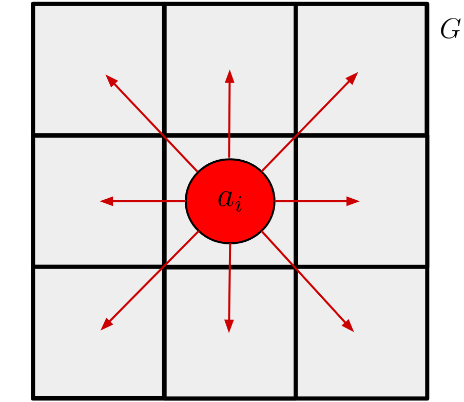
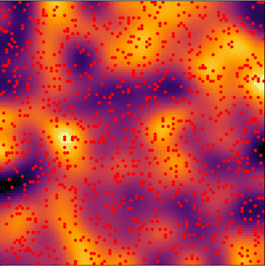
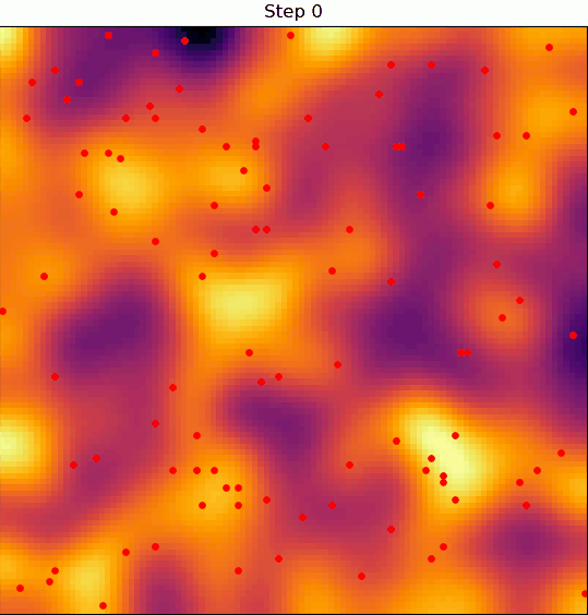
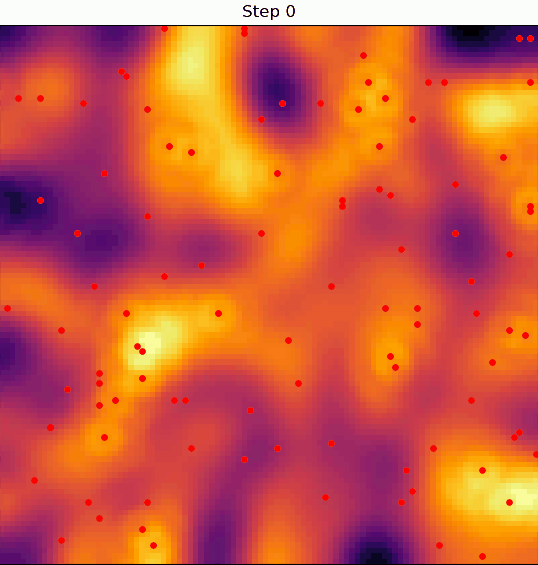
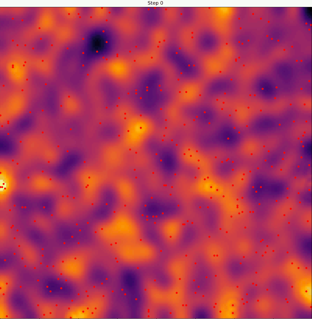
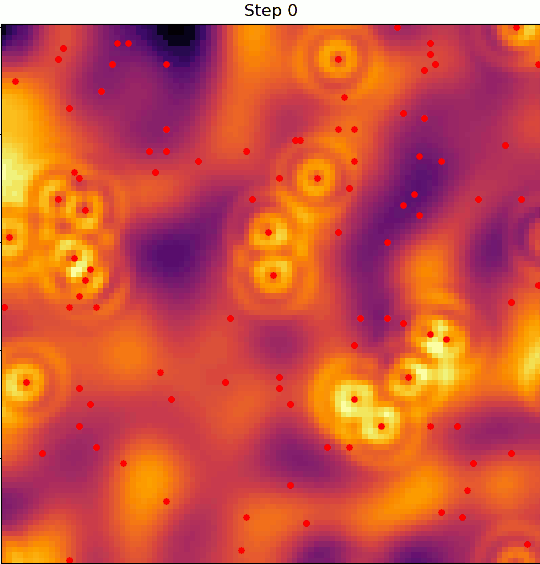
We'll be building an agent-based model, i.e. a model where a discrete number of nomads (agents) move throughout space and interact with each other and with the local terrain in some way. At any given moment in time, an agent will look at their surroundings and decide whether the land on which they're situated is good enough for them to settle or not. If it is, then they'll stop wandering, settle in, and form a "village"; if not, they'll continue wandering in search of better land. Here's where things get interesting: a village can degrade the quality of the land it sits on. If that land degrades enough, the nomad that settled in that village can decide to disband it and continue on wandering. So, the dynamics evolve under two-way coupling: the terrain quality determines whether villages form, and the presence of villages determines the quality of the terrain.

Version 1: first steps

The dynamics of our model will unfold on a static, structured 2D spatial grid \( G = \lbrace \mathbf{g_{ij}} \rbrace \), where \( \mathbf{g_{ij}}=(x_i,y_j) \) with \( i = 1 \dots n_x \) and \( j = 1 \dots n_y \). We'll describe agents by their location on \(G\): \( A = \lbrace \mathbf{a_i} \rbrace \; \text{for} \; i=1 \dots n_a \), where \(\mathbf{a_i} \in G\). Villages will also be characterized in this way: \( V = \lbrace \mathbf{v_i} \rbrace \; \text{for} \; i=1 \dots n_v \), where \( \mathbf{v_i} \in G \). The terrain quality \( T(x,y) : \mathbb{R}^2 \mapsto \mathbb{R} \) is a spatial field defined on \( G \).

With those basic definitions out of the way, let's talk about how the agents move about. At any given moment in time, agent \(a_i\) evaluates the quality of their terrain \( T(\mathbf{a_i}) \). If \( T(\mathbf{a_i}) \ge T^* \), then that agent "settles" to form a village. Algorithmically, this means that we pop the location \( \mathbf{a_i} \) off of the set \(A\) and append it to the set \(V\). Otherwise, \( T(\mathbf{a_i}) < T^* \), and the agent continues to wander. This wandering is modeled as a random process: the agent randomly chooses one of the 8 grid locations that neighbor \(\mathbf{a_i}\), call it \( \mathbf{a_i^*} \). If \( T(\mathbf{a_i^*}) > T(\mathbf{a_i}) \), then the agent moves to this "better" square; otherwise, it stays put with some probability. If it so happens that the agent stumbles onto a pre-existing village, they will just automatically decide to settle there.

This is sufficient to define a "version 1" of our model; see below for an example simulation of it.

The terrain quality \( T(x,y) \) is represented in the inferno colorscale, with yellower colors being better. The simulation is initialized with randomly placed agents, and these wander about. We see the evolution of a long-term steady state: statistically speaking, the agents simply trace out the level set defined by \( T(x,y) = T^* \).

Version 2: villages spawn new nomads

The first addition we'll make is to allow villages to randomly spawn new agents with some probability.

This looks pretty similar to the previous version; the only difference is that the steady state is now defined by \( T(x,y) \ge T^* \). This is because of the new agents which spawn: previously, most of the villages were formed by agents who wandered progressively "uphill" toward yellower areas. These agents would settle as soon as they hit a location with a desirability on the \( T^* \) threshold. This still happens, but now, new agents can sometimes spawn at locations where \( T(x,y) > T^* \), which pushes the local front of villages "inward" until the entire blob of desirable terrain is occupied.

Version 3: terrain degradation from village overpopulation

Now we introduce a more interesting dynamic by coupling the terrain to the villages. The general idea is that if a local area is heavily populated with villages, then the resources should start to deplete and \( T(x,y) \) should decrease. We also allow for a resource-depleted area to regenerate over time, at a rate proportional to how depleted it is. This gives the following discrete time update rule for \( T(x,y) \): \[ T_{\mathbf{g_{ij}}} \mapsto T_{\mathbf{g_{ij}}} - c_1 f_d( V , \mathbf{g_{ij}} ) + c_2 ( 1 - T_{\mathbf{g_{ij}}} ) \]

where \( T_{\mathbf{g_{ij}}} \) denotes \(T\) at grid location \(\mathbf{g_{ij}}\) and \( f_d(V,\mathbf{g_{ij}}) \) is a function that estimates the density of villages at \( \mathbf{g_{ij}} \).

There are several conceivable choices for the density function. One intuitive definition to consider is to average the number of villages in the vicinity of a grid point using a Gaussian weighting. This choice is natural for estimating local properties since it places highest weight at central locations. The density about a central point \( \mathbf{g_{ij}} \) can be estimated by simply "counting" the number of villages in the vicinity, weighting each of them by the Gaussian centered at \( \mathbf{g_{ij}} \). We can write this as: \[ f_d(V,\mathbf{g_{ij}}) = \int_{\mathbf{x}} \mathbb{1}_v(\mathbf{x}) \mathcal{N}_{\sigma}( \| \mathbf{x} - \mathbf{g_{ij}} \| ) d\mathbf{x} \] where \( \mathbb{1}_v(\cdot) \) is the one-indicator function; it tells you whether or not a village is present at a given location. Notice this is the same as convolution with a kernel: \[ f_d(V,\mathbf{g_{ij}}) = ( \mathbb{1}_v \star k )(\mathbf{g_{ij}}) \] where, in this particular case, we've chosen the kernel to be Gaussian, i.e. \( k(\cdot) = \mathcal{N}_{\sigma}( \cdot ) \).

Writing the density function as a convolution is a good idea for a couple reasons. First, it gives us a very convenient way to calculate it, since lots of libraries already exist for computing convolutions (especially these days with ML/AI). Second, it motivates the question: what about other choices of kernel? One thing that might be fun to do is to consider a kernel that in some sense has an opposite effect to that of a Gaussian. So, what's the general effect of a Gaussian kernel?

To answer that question, it helps to introduce a bit of math, and connect kernels to the theory of partial differential equations (PDEs). It turns out that the Gaussian kernel is the Green's function of the heat equation: \[ u_t = \nu \nabla^2 u \] A consequence of this is that the heat equation can be solved, given any initial condition, by convolution with a Gaussian kernel. What this means for us is that there will be a deep connection between the behavior of our agent-based system and that of the heat equation. We know that the heat equation produces very smooth solutions: sharp features are dulled down and everything sort of regresses to a global, boring average.

So, the kernel we chose smooths things out. What's the opposite of that? Motivated by the PDE theory we just discussed, we can "work backwards", starting with a PDE that we know has different behavior and asking what its Green's function is. The Helmholtz equation is a good candidate in this regard: \[ (\nabla^2 - w^2)u = \delta(\mathbf{x}) \] Instead of smoothing, this equation tends to produce sharply defined, resonant spatial wavelengths. Its Green's function can be approximated by cosine-ripple functions that look like this: \[ k_h( \| \mathbf{x} - \mathbf{g_{ij}} \| ) = \text{cos}(w \| \mathbf{x} - \mathbf{g_{ij}} \| ) \; \text{exp}\left[ -\| \mathbf{x} - \mathbf{g_{ij}} \|^2 / 2 \sigma^2 \right] \]

So, we can create a density function that combines these kernels: \[ f_d(V,\mathbf{g_{ij}}) = ( \mathbb{1}_v \star (\alpha k_d + \beta k_h) )(\mathbf{g_{ij}}) \] where \( k_d \) and \( k_h \) are the diffusion (heat) and Helmholtz kernels, respectively. With this combination, we can pit these two kernels against each other, producing dynamics that are a compromise between their opposing effects.

To see this, let's take a look below at what the behavior looks like for different combinations of diffusion and resonance.

We see pretty clearly that which we just explored in the abstract. When the terrain degrades under the action of a pure diffusive kernel, everything smooths out, and the terrain field \( T(x,y) \) is driven to a very uniform state. This lack of spatial differentiation results "feast or famine" cycles, in which we observe either the formation of lots of villages everywhere, or very few villages anywhere. Diffusion is thus something of an egalitarian operator, driving every corner of the grid to more or less the same global state.

The Helmholtz ripple kernel is clearly very much the opposite. We see that under its influence, a few tightly clustered "kingdoms" develop and strengthen in power and influence, so much so that a global steady state consisting of one single village cluster emerges. And so, we have the yin-and-yang opposition which we sought. A Gaussian is egalitarian, a ripple is elitist; diffusion favors chaos, Helmholtz favors order.

The final plot in the group of three above shows a glimpse of the sort of beauty that emerges when you combine these two forces. Kingdoms rise and fall; vagabonds disband and re-consolidate.

Final version

We'll add a couple other cosmetic effects to this version, but the basic core will be driven by the competition between diffusion and resonance that we saw previously. First: adding some external forcing to \( T(x,y) \) can make things interesting. So, we'll randomly perturb \( T(x,y) \) every so often with a Gaussian at a randomly chosen location. We'll also add some vortices at fixed locations to swirl things around: \[ T_{\mathbf{g_{ij}}} \mapsto T_{\mathbf{g_{ij}}} - \mathbf{v} \cdot \frac{dT_{\mathbf{g_{ij}}}}{d\mathbf{x}} \Delta t \]

Here, \( \mathbf{v} = (v_x,v_y) \) is the velocity field imposed by a vortex swirling at a fixed spatial location: \[ v_x = -\frac{ r_y }{ r } \; , \; v_y = \frac{ r_x }{ r } \] where \( r = \| \mathbf{x} - \mathbf{x_0} \| \) is the distance to the vortex center.

Other than that, we'll introduce another mode to simulate village collapse from local overpopulation. This will work in a similar fashion to how we modeled terrain degradation, by convolving \( T(x,y) \) with a Gaussian. The difference is that here, we directly collapse villages based on local density: \[ v_{\mathbf{g_{ij}}} \mapsto \emptyset \; \text{if} \; \xi < \frac{c_1}{ 1 + \text{exp}[ -(f_d(\mathbf{g_{ij}}) - c_2) / c_3 ] } \] Where \( \xi \sim \mathcal{U}[0,1] \) is just a uniform random number, and \( f_d(\cdot) \) is computed with a (normalized) Gaussian kernel, so that it represents local village density.

Parting thoughts

There's a lot here that I find fascinating. Probably top of the list is the concept of emergence, and how complex, large scale behavior can self-organize from fairly simple rules at the small scales. In these simulations, we see this manifest as the competition that evolves between the order-imposing ripple kernel and the diffusive kernel. It's an interesting lesson in how sometimes, really beautiful behavior is the product of a fight between opposing forces.

Another prominent duality is stasis versus flow. Clearly, all agents want to settle into a permanent village, but the very act of doing so depletes the resources on which their village stands, making it less stable over time. This is of course exacerbated by the fact that all agents want the same thing, which leads to overpopulation. So you get a global population that is constantly going through cycles: for a stretch, things might seem pretty ordered and static, only to be followed by an equally long period of reshuffling and migration. Nature seems to be playing with these poor nomads, who look like they're always just a couple steps behind it, always chasing the nearest shiny patch of land, only to have to start all over just as soon as they reach it.